Predicting Survival Times from Alone

Introduction

Today I’ll explore another interesting #tidytuesday data set consisting of data from the TV show Alone. For those not familiar with the show, 10 contestants are dropped off in a remote location in the wilderness with limited supplies. They attempt to survive for as long as they can until they tap out, and the last man standing wins a significant cash prize.

The data has its own R package. The package as well as more information about the data can be found here.

The goal of this analysis is to explore and model the factors that predict how long a competitor will survive.

Data Exploration

Data Ingest

First let’s import the data for our survivalists and the locations. I will be using the static data set from github since the package data changes over time and I want to avoid breaking any code.

library(tidyverse)
library(alone)

data(survivalists)
data(seasons)
data(loadouts)

# survivalists2 <- read_csv('https://raw.githubusercontent.com/rfordatascience/tidytuesday/master/data/2023/2023-01-24/survivalists.csv')
# loadouts2 <- read_csv('https://raw.githubusercontent.com/rfordatascience/tidytuesday/master/data/2023/2023-01-24/loadouts.csv')
# seasons2 <- read_csv('https://raw.githubusercontent.com/rfordatascience/tidytuesday/master/data/2023/2023-01-24/seasons.csv')

survivalists <- 
  survivalists |> 
  filter(season <= 9, version == "US")
  
loadouts <- 
  loadouts |> 
  filter(season <= 9, version == "US")

seasons <- 
  seasons |> 
  filter(season <= 9, version == "US")

glimpse(survivalists)

Rows: 94
Columns: 20
$ version             <chr> "US", "US", "US", "US", "US", "US", "US", "US", "U…
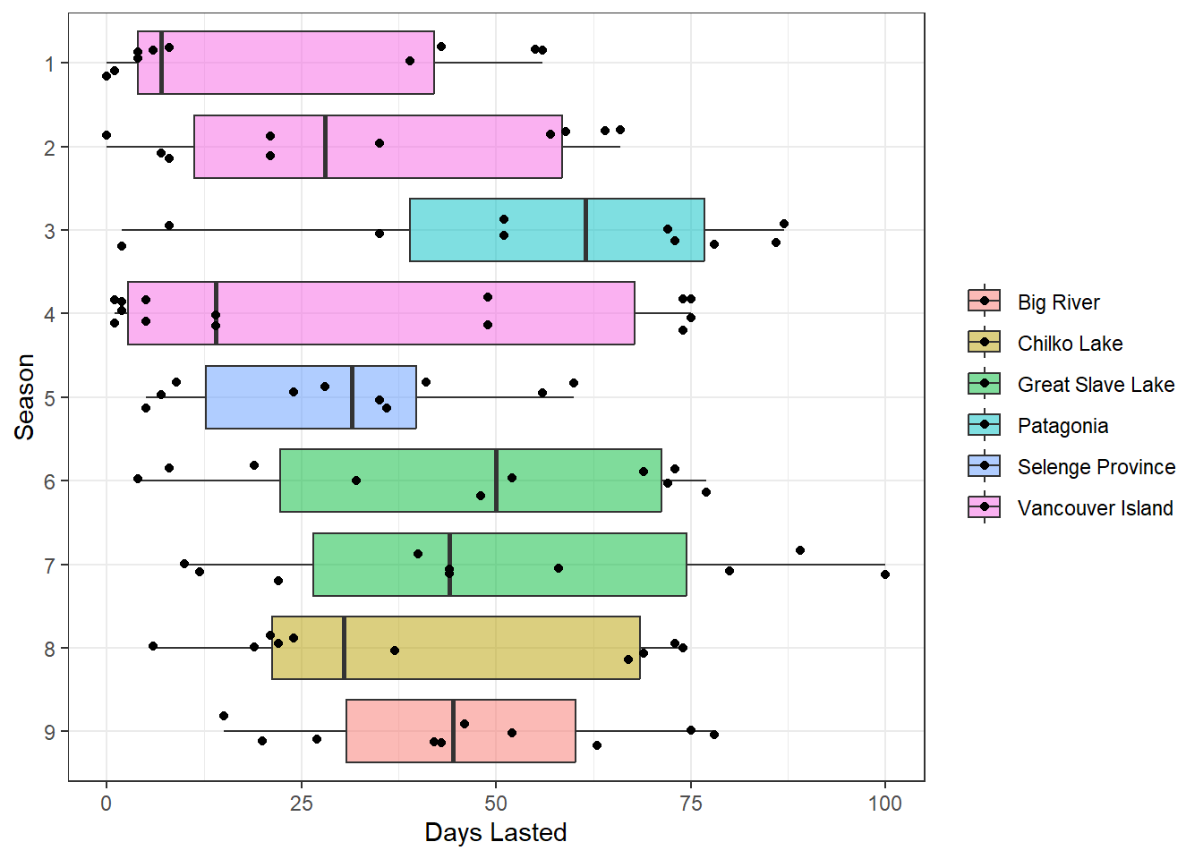
$ season              <dbl> 1, 1, 1, 1, 1, 1, 1, 1, 1, 1, 2, 2, 2, 2, 2, 2, 2,…
$ id                  <chr> "US010", "US009", "US008", "US007", "US006", "US00…
$ name                <chr> "Alan Kay", "Sam Larson", "Mitch Mitchell", "Lucas…
$ first_name          <chr> "Alan", "Sam", "Mitch", "Lucas", "Dustin", "Brant"…
$ last_name           <chr> "Kay", "Larson", "Mitchell", "Miller", "Feher", "M…
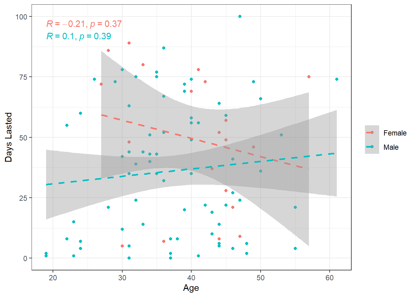
$ age                 <dbl> 40, 22, 34, 32, 37, 44, 46, 24, 41, 31, 50, 44, 45…
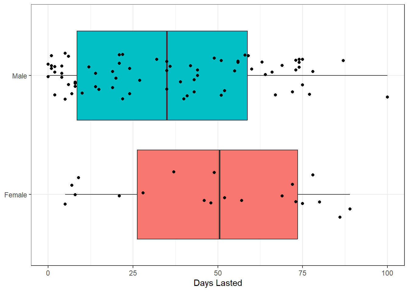
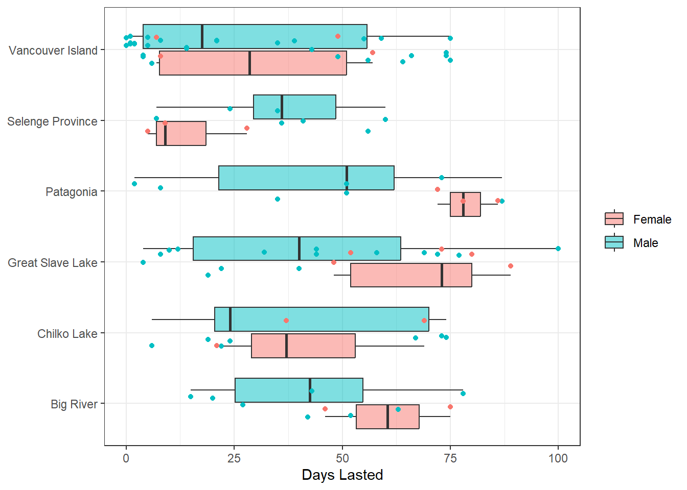
$ gender              <chr> "Male", "Male", "Male", "Male", "Male", "Male", "M…
$ city                <chr> "Blairsville", "Lincoln", "Bellingham", "Quasqueto…
$ state               <chr> "Georgia", "Nebraska", "Massachusetts", "Iowa", "P…
$ country             <chr> "United States", "United States", "United States",…
$ result              <dbl> 1, 2, 3, 4, 5, 6, 7, 8, 9, 10, 1, 2, 3, 4, 5, 6, 7…
$ days_lasted         <dbl> 56, 55, 43, 39, 8, 6, 4, 4, 1, 0, 66, 64, 59, 57, …
$ medically_evacuated <lgl> FALSE, FALSE, FALSE, FALSE, FALSE, FALSE, FALSE, F…
$ reason_tapped_out   <chr> NA, "Lost the mind game", "Realized he should actu…
$ reason_category     <chr> NA, "Personal", "Personal", "Personal", "Personal"…
$ episode_tapped      <dbl> NA, NA, NA, NA, NA, NA, NA, NA, 2, 1, NA, NA, NA, …
$ team                <chr> NA, NA, NA, NA, NA, NA, NA, NA, NA, NA, NA, NA, NA…
$ day_linked_up       <dbl> NA, NA, NA, NA, NA, NA, NA, NA, NA, NA, NA, NA, NA…
$ profession          <chr> "Corrections Officer", "Outdoor Gear Retailer", "B…

days_lasted is the variable we are most interested in and the one we will try to predict. Furthermore, we aren’t interested in any variable that isn’t known at the start of the season (i.e. reason_tapped_out)

Gender

How many men vs. women have attempted the show?

survivalists |> count(gender)

# A tibble: 2 × 2
  gender     n
  <chr>  <int>
1 Female    20
2 Male      74

Looks like there are about 4 times as many men as there are women. How do men and women compare in their survival times?

survivalists |> 
  ggplot(aes(gender, days_lasted)) +
  geom_boxplot(aes(fill = gender), show.legend = F) +
  geom_jitter(width = .2, height = 0) +
  coord_flip() +
  labs(x = NULL, y = "Days Lasted", fill = NULL)

Women in this show appear to have a slight survival advantage.

Location

How do survival times compare by season and location?

survivalists |> 
  left_join(seasons |> select(season, location)) |> 
  mutate(season = fct_reorder(factor(season), -season)) |> 
  ggplot(aes(season, days_lasted, fill = location)) +
  geom_boxplot(alpha = .5) +
  geom_jitter(width = .2, height = 0) +
  coord_flip() +
  labs(x = "Season", y = "Days Lasted", fill = NULL)

If you look closely, you’ll notice that season 4 competitors drop out in pairs. That’s because the competitors were put in teams in this season. We’ll be sure to account for that when we model.

Finally, let’s compare gender survival times by location

survivalists |> 
  left_join(seasons |> select(season, location)) |> 
  ggplot(aes(location, days_lasted, fill = gender)) +
  geom_boxplot(alpha = .5) +
  geom_jitter(aes(color = gender), width = .2, height = 0, show.legend = F) +
  coord_flip() +
  labs(x = NULL, y = "Days Lasted", fill = NULL, color = NULL)

For some locations, women greatly out-survive men. Others, not so much.

Age

How does age correlate with survival?

survivalists |> 
  ggplot(aes(age, days_lasted, color = gender)) +
  geom_point() +
  geom_smooth(method = "lm", lty = 2) +
  labs(x = "Age", y = "Days Lasted", color = NULL) +
  ggpubr::stat_cor(show.legend = F) 

There doesn’t appear to be an age effect.

Items

Let’s import one more data set that consists of the items the survivalists bring with them on the show.

library(patchwork)

ridges <- 
  loadouts |>
  left_join(survivalists |> select(name, season, days_lasted)) |>
  add_count(item) |>
  mutate(
    item = fct_lump_min(item, min = 3),
    item = fct_reorder(item, n)
  ) |>
  ggplot(aes(days_lasted, item)) +
  ggridges::geom_density_ridges(aes(fill = item), panel_scaling = F, show.legend = F, alpha = .8) +
  labs(x = "Days Lasted", y = NULL)

totals <-
  loadouts |> 
  mutate(item = fct_lump_min(item, min = 3)) |>
  count(item) |> 
  mutate(item = fct_reorder(item, n)) |> 
  mutate(item = fct_relevel(item, "Other", after = 0)) |> 
  ggplot(aes(item, n)) +
  geom_col(alpha = .8, aes(fill = item), show.legend = F) +
  geom_label(aes(label = n), size = 3) +
  coord_flip() +
  labs(y = "Total", x = NULL) +
  theme(axis.text.y = element_blank(), axis.ticks.y = element_blank())

ridges + totals

While it’s difficult to infer anything from these charts, there is evidence that items do have an effect on survival.

Repeated Contestants

We should also investigate the fact that in season 5, each contestant was a repeat survivalist. We should look at how each of them fared from their first attempt to their second.

survivalists |> 
  left_join(seasons |> select(season, location)) |> 
  filter(n() > 1, .by = name) |> 
  mutate(
    attempt = str_glue("Attempt {rank(season)}"), 
    slope = (days_lasted[attempt == "Attempt 1"] - days_lasted[attempt == "Attempt 2"]) / 2,
    .by = name, days_lasted, location, .keep = "used"
  ) |>
  ggplot(aes(attempt, days_lasted, group = name)) + 
  geom_point(aes(shape = location), size = 2) +
  geom_line(aes(color = slope > 0)) +
  scale_color_manual(values = c("#00b545", "red"), labels = c("Survived Longer", "Survived Shorter")) +
  labs(title = "Repeat Survivalists", x = NULL, y = "Days Lasted", shape = "Location", color = "2nd Attempt")

It’s interesting that only roughly half of them survived longer on their 2nd attempt even accounting for location of their first attempt.

Prior Survival Experience

Lastly, let’s look at how profession might affect survival time. Some contestants are “Survival Experts” or “Hunting Guides”. So we will label them to have “Prior Experience”.

survivalists |> 
  mutate(prior_experience = profession |> str_detect("Surv|Wilderness|Hunt|Outdoor|Skills|Instructor")) |> 
  ggplot(aes(prior_experience, days_lasted)) + 
  geom_boxplot(aes(fill = prior_experience), alpha = .5) +
  ggrepel::geom_text_repel(
    aes(label = profession), 
    direction = "y",
    min.segment.length = 50,  
    max.overlaps = 50, 
    position = position_jitter(width = .2, height = 0), 
    size = 2
  ) +
  coord_flip() +
  labs(x = "Prior Experience", y = "Days Lasted") +
  theme(legend.position = "none")

Machine Learning

Let’s build a model to predict survival time!

First, we will prepare our data by selecting the necessary variables. We’ll have to pivot the items data to get it into wide format so we can join with our survivalists data set.

items_wide <- 
  loadouts |> 
  mutate(item = fct_lump_min(item, min = 3)) |>
  mutate(present = 1) |> 
  pivot_wider(
    id_cols = c(name, season), 
    names_from = item, 
    values_from = present,
    values_fn = first,
    values_fill = 0,
    names_prefix = "item_"
  )

alone_clean <-
  survivalists |> 
  left_join(seasons |> select(season, location)) |> 
  left_join(items_wide) |> 
  mutate(repeat_attempt = rank(season) > 1, .by = name) |> 
  select(
    name, season, age, gender, location, days_lasted, team, country, profession, repeat_attempt, 
    starts_with("item_")
  )

Train/Test Sets

Next we will create our train/test sets, as well as some resamples. Since our data set is so small, we will use bootstrap resampling and we will stratify by season to ensure we sample across different survival conditions.

library(tidymodels)

set.seed(234)
alone_split <- initial_split(alone_clean, strata = season)
alone_train <- training(alone_split)
alone_test <- testing(alone_split)

alone_boot <- bootstraps(alone_train, times = 10, strata = season)

Feature Engineering

Moving on to our feature engineering, we will create a few of the variables we’ve already explored.

One of my favorite pre-processing techniques to use when data includes a grouping structure is step_lencode_mixed() from the {embed} package. This step assigns a numeric value to our location variable by training a simple mixed model using the {lme4} package. This is better than dummy encoding because it accounts for differing group counts and will automatically assign a value close to the mean when a new location is encountered. Plus, it doesn’t increase the number of dimensions of the data set as dummy encoding would.

alone_rec <- 
  recipe(
    days_lasted ~ .,
    data = alone_train
  ) |> 
  update_role(name, new_role = "id") |> 
  update_role(season, new_role = "season_id") |> 
  step_mutate(
    prior_experience = profession |> stringr::str_detect("Surv|Wilderness|Hunt|Outdoor|Skills|Instruct"),
    US_orig = country == "United States",
    team = !is.na(team),
    across(where(is.logical), factor)
  ) |> 
  embed::step_lencode_mixed(location, outcome = vars(days_lasted)) |> 
  step_rm(profession, country) |> 
  step_dummy(all_factor_predictors())

Model Training/Tuning

Let’s train a random forest regression model. We will tune and optimize for RMSE. Since it’s a small data set, we will stick with relatively small numbers of trees.

rf_spec <- 
  rand_forest(mtry = tune(), trees = tune()) |>
  set_engine("ranger") |> 
  set_mode("regression")

alone_wf <-
  workflow() |>
  add_recipe(alone_rec) |>
  add_model(rf_spec)

rf_grid <- 
  grid_regular(
    mtry(c(5, 25)), 
    trees(c(10, 100)), 
    levels = c(mtry = 5, trees = 10)
  )

doParallel::registerDoParallel()

alone_res <-
  alone_wf |>
  tune_grid(
    resamples = alone_boot,
    grid = rf_grid,
    control = control_resamples(allow_par = T, parallel_over = "everything")
  )

alone_res |> autoplot()

Turns out this is a very hard problem to predict. Nevertheless, we will pick our best model and do one last fit.

best_params <- alone_res |> select_best(metric = "rmse")

set.seed(678)

alone_final <- 
  alone_wf |> 
  update_model(rand_forest(mode = "regression") |> set_engine("ranger", importance = "permutation")) |>
  finalize_workflow(best_params) |> 
  last_fit(alone_split)

Results

Final Performance Metrics

alone_final |> collect_metrics()

# A tibble: 2 × 4
  .metric .estimator .estimate .config             
  <chr>   <chr>          <dbl> <chr>               
1 rmse    standard      27.3   Preprocessor1_Model1
2 rsq     standard       0.186 Preprocessor1_Model1

Looks like the final model’s metrics were slightly better than our cross-validated metrics. This is probably because we got to train on the full training set.

Predictions

Now we will compare our predictions against the true values from the test set. The dotted black line represents the formula y = x, which is where we’d hope all our predictions would lie.

alone_final |> 
  collect_predictions() %>%
  inner_join(alone_clean |> slice(.$.row)) |> 
  ggplot(aes(.pred, days_lasted)) +
  geom_point(aes(color = location, shape = location), size = 2) +
  geom_abline(slope = 1, intercept = 0, lty = 2) +
  labs(shape = NULL, color = NULL, x = "Predicted Days Lasted", y = "Actual Days Lasted") +
  expand_limits(x = 0, y = 0)

The good news is that there doesn’t appear to be a whole lot of bias in our model (no systematic under or over predicting). However, our predictions tend to be quite far off most of the time.

Variable Importance

To finish things off, we’ll look at the variable importances tracked by our model. It’s important to note that permutation importance doesn’t indicate direction of effect, only magnitude. Nonetheless, we can infer the probable direction by looking back at our EDA plots.

alone_final |> 
  extract_fit_engine() |>
  vip::vip(n = 20)

Unsurprisingly we see that gender and location affect survival time. Interestingly, there are a few not so obvious items that appear to affect survival time. Perhaps trapping wire is a must to survive in the wild!

Conclusion & Discussion

After exploring and modeling this data set, it’s clear that it’s quite difficult to predict how long contestants will last on the show. There are likely two main reasons for this. The first is that our sample is so limited. 9 seasons with 10 contestants each is no where near enough to extract robust and meaningful patterns. The second reason is that we don’t have enough data on the existing contestants. Additional information that could be helpful include relationship status/family info, personality characteristics, and socio-economic status.

More detailed data about the locations could be helpful as well, such as time of year and weather patterns at drop-off time. Perhaps some of this information could be acquired from actually watching the show.

There’s also the fact that there is likely some inconsistent bias that the producers of the show introduce when they select contestants. It’s very possible that they select people differently each season based on viewership and popularity of prior seasons. This makes it difficult to detect potential patterns across seasons.