Visualizing NFL Game Attendance

Photo by Anders Krøgh Jørgensen on Unsplash

In this blog post we will be visualizing potential factors that drive NFL game attendance. The data come from a #TidyTuesday data set from 2020 which consists of game attendance data between the years 2000 and 2019. I also managed to track down another data set from Kaggle that includes useful data about stadiums and weather.

Data Import

We start off by loading the tidyverse and importing the data. In this analysis, we will only be looking at regular season games.

library(tidyverse) # loads all our favorite data analysis packages
theme_set(theme_bw()) # make all our plots look a little nicer

Attendance

attendance <-
  read_csv(
    "https://raw.githubusercontent.com/rfordatascience/tidytuesday/master/data/2020/2020-02-04/attendance.csv",
    col_select = c(team, team_name, year, week, weekly_attendance)
  ) |>
  drop_na(weekly_attendance) # remove bye weeks

attendance |> glimpse()

Rows: 10,208
Columns: 5
$ team              <chr> "Arizona", "Arizona", "Arizona", "Arizona", "Arizona…
$ team_name         <chr> "Cardinals", "Cardinals", "Cardinals", "Cardinals", …
$ year              <dbl> 2000, 2000, 2000, 2000, 2000, 2000, 2000, 2000, 2000…
$ week              <dbl> 1, 2, 4, 5, 6, 7, 8, 9, 10, 11, 12, 13, 14, 15, 16, …
$ weekly_attendance <dbl> 77434, 66009, 71801, 66985, 44296, 38293, 62981, 352…

Games

conferences <-
  read_csv(
    "nfl_teams.csv",
    col_select = c(team_name, conference = team_conference)
  )

games <-
  read_csv("https://raw.githubusercontent.com/rfordatascience/tidytuesday/master/data/2020/2020-02-04/games.csv") |>
  # fixing error in the data
  rows_update(
    tibble(
      year = 2005,
      week = "2",
      winner = "New York Giants",
      home_team = "New York Giants",
      away_team = "New Orleans Saints"
    ),
    by = c("year", "week", "winner")
  )

game_details <-
  read_csv(
    "spreadspoke_scores.csv",
    col_select = c(
      week = schedule_week, year = schedule_season,
      home_team = team_home, away_team = team_away, stadium,
      weather_temperature # select the few columns I need
    )
  )

games <-
  games |>
  left_join(game_details) |>
  mutate(week = as.numeric(week)) |> # non-regular weeks are not numeric and get converted to NA
  drop_na(week) # drop non-regular games

games |> glimpse()

Rows: 5,104
Columns: 21
$ year                <dbl> 2000, 2000, 2000, 2000, 2000, 2000, 2000, 2000, 20…
$ week                <dbl> 1, 1, 1, 1, 1, 1, 1, 1, 1, 1, 1, 1, 1, 1, 1, 2, 2,…
$ home_team           <chr> "Minnesota Vikings", "Kansas City Chiefs", "Washin…
$ away_team           <chr> "Chicago Bears", "Indianapolis Colts", "Carolina P…
$ winner              <chr> "Minnesota Vikings", "Indianapolis Colts", "Washin…
$ tie                 <chr> NA, NA, NA, NA, NA, NA, NA, NA, NA, NA, NA, NA, NA…
$ day                 <chr> "Sun", "Sun", "Sun", "Sun", "Sun", "Sun", "Sun", "…
$ date                <chr> "September 3", "September 3", "September 3", "Sept…
$ time                <time> 13:00:00, 13:00:00, 13:01:00, 13:02:00, 13:02:00,…
$ pts_win             <dbl> 30, 27, 20, 36, 16, 27, 21, 14, 21, 41, 9, 23, 20,…
$ pts_loss            <dbl> 27, 14, 17, 28, 0, 7, 16, 10, 16, 14, 6, 0, 16, 13…
$ yds_win             <dbl> 374, 386, 396, 359, 336, 398, 296, 187, 395, 425, …
$ turnovers_win       <dbl> 1, 2, 0, 1, 0, 0, 1, 2, 2, 3, 0, 1, 1, 0, 3, 4, 1,…
$ yds_loss            <dbl> 425, 280, 236, 339, 223, 249, 278, 252, 355, 167, …
$ turnovers_loss      <dbl> 1, 1, 1, 1, 1, 1, 1, 3, 4, 2, 4, 6, 2, 1, 0, 1, 3,…
$ home_team_name      <chr> "Vikings", "Chiefs", "Redskins", "Falcons", "Steel…
$ home_team_city      <chr> "Minnesota", "Kansas City", "Washington", "Atlanta…
$ away_team_name      <chr> "Bears", "Colts", "Panthers", "49ers", "Ravens", "…
$ away_team_city      <chr> "Chicago", "Indianapolis", "Carolina", "San Franci…
$ stadium             <chr> "Hubert H. Humphrey Metrodome", "Arrowhead Stadium…
$ weather_temperature <dbl> 72, 86, 76, 72, 73, 75, 63, 72, 78, 95, 60, 84, 69…

Stadiums

stadiums <-
  read_csv(
     "nfl_stadiums.csv",
    col_select = c(
     stadium = stadium_name, stadium_capacity, stadium_latitude,
     stadium_longitude, stadium_address, stadium_open, stadium_type
    )
  ) |>
  mutate(
    stadium_id = cur_group_id(), # Some stadiums were renamed at various points. We want to group those together
    .by = c(stadium_address, stadium_open),
    .before = 1
  ) |>
  select(-stadium_address, stadium_open)

stadiums |> glimpse()

Rows: 120
Columns: 7
$ stadium_id        <int> 1, 2, 3, 4, 4, 5, 6, 7, 8, 9, 10, 11, 12, 13, 14, 15…
$ stadium           <chr> "Acrisure Stadium", "Alamo Dome", "Allegiant Stadium…
$ stadium_capacity  <dbl> 65500, 72000, 65000, 75024, NA, NA, NA, 76416, 80000…
$ stadium_latitude  <dbl> 40.48460, 29.41694, 36.09075, NA, 30.32389, NA, NA, …
$ stadium_longitude <dbl> -80.21440, -98.47889, -115.18372, NA, -81.63750, NA,…
$ stadium_open      <dbl> 2001, NA, 2020, NA, NA, NA, 1980, 1972, 2009, 1966, …
$ stadium_type      <chr> "outdoor", "indoor", "indoor", "outdoor", NA, "outdo…

These tibbles contain fairly basic info about each game. including who was playing, who won, which stadium the game was at, and most importantly, the game attendance. For this analysis, game statistics such as points scored are largely irrelevant since game attendance is determined at the beginning of game. That being said, past performance might be indicative of future attendance which we will explore later.

Data Transformation

Since the attendance tibble doesn’t contain information about which team is home or away, we’ll need to join it with the games tibble based on team, year, and week. This appears trivial at first, but actually requires us to pivot the games tibble in order to create a single column for team name that we can join with attendance.

# select variables of interest from attendance
attendance_simple <-
  attendance |>
  mutate(team_name = paste(team, team_name)) |>
  select(week, year, team_name, weekly_attendance)

# determine loser and select variables of interest
games_long <-
  games |>
  mutate(
    loser = if_else(winner == home_team, away_team, home_team)
  ) |>
  pivot_longer(c(home_team, away_team), names_to = "home_away", values_to = "team_name") |>
  select(team_name, home_away, winner, loser, week, year)



attendance_joined <-
  attendance_simple |>
  inner_join(games_long) |>
  inner_join(conferences) |>
  arrange(team_name, year, week)

attendance_joined |>
  glimpse()

Rows: 10,208
Columns: 8
$ week              <dbl> 1, 2, 4, 5, 6, 7, 8, 9, 10, 11, 12, 13, 14, 15, 16, …
$ year              <dbl> 2000, 2000, 2000, 2000, 2000, 2000, 2000, 2000, 2000…
$ team_name         <chr> "Arizona Cardinals", "Arizona Cardinals", "Arizona C…
$ weekly_attendance <dbl> 77434, 66009, 71801, 66985, 44296, 38293, 62981, 352…
$ home_away         <chr> "away_team", "home_team", "home_team", "away_team", …
$ winner            <chr> "New York Giants", "Arizona Cardinals", "Green Bay P…
$ loser             <chr> "Arizona Cardinals", "Dallas Cowboys", "Arizona Card…
$ conference        <chr> "NFC", "NFC", "NFC", "NFC", "NFC", "NFC", "NFC", "NF…

Now that we’ve joined attendance and games together, we need to pivot back to “wide” format to achieve “tidyness”. Before we do that, let’s calculate win streak and lose streaks for each team at the time of the match up. To do this we will use the rle function, which calculates run length encodings of equal values in a vector. This solution admittedly feels kinda hacky since it’s not a traditional tidyverse function, but it’s the best way I could find. Please let me know if you know of a better way!

streaks <-
  attendance_joined |>
  group_by(
    team_name,
    winner_grp = with(rle(winner), rep(seq_along(lengths), lengths))
  ) |>
  mutate(
    win_streak = seq_along(winner_grp) - 1,
  ) |>
  group_by(
    team_name,
    loser_grp = with(rle(loser), rep(seq_along(lengths), lengths))
  ) |>
  mutate(
    lose_streak = seq_along(loser_grp) - 1
  ) |>
  ungroup() |>
  select(-winner_grp, -loser_grp) |>
  pivot_wider(
    names_from = home_away,
    values_from = c(team_name, win_streak, lose_streak, conference)
  ) |>
  rename(
    away_team = team_name_away_team,
    home_team = team_name_home_team
  )

To finish off our tidy data set, we will join in the stadium and temperature data.

nfl_tidy <-
  streaks |>
  left_join(
    games |>
      select(week, year, home_team, away_team, stadium, weather_temperature)
  ) |>
  left_join(stadiums) |>
  # rename all stadiums to what they are currently named
  mutate(stadium = stadium[which.max(year)], .by = stadium_id)

nfl_tidy |> glimpse()

Rows: 5,104
Columns: 21
$ week                  <dbl> 1, 2, 4, 5, 6, 7, 8, 9, 10, 11, 12, 13, 14, 15, …
$ year                  <dbl> 2000, 2000, 2000, 2000, 2000, 2000, 2000, 2000, …
$ weekly_attendance     <dbl> 77434, 66009, 71801, 66985, 44296, 38293, 62981,…
$ winner                <chr> "New York Giants", "Arizona Cardinals", "Green B…
$ loser                 <chr> "Arizona Cardinals", "Dallas Cowboys", "Arizona …
$ away_team             <chr> "Arizona Cardinals", "Dallas Cowboys", "Green Ba…
$ home_team             <chr> "New York Giants", "Arizona Cardinals", "Arizona…
$ win_streak_away_team  <dbl> 0, 0, 1, 0, 0, 0, 0, 3, 0, 0, 0, 0, 0, 0, 5, 0, …
$ win_streak_home_team  <dbl> 0, 0, 0, 1, 0, 0, 0, 0, 0, 0, 2, 0, 0, 3, 0, 0, …
$ lose_streak_away_team <dbl> 0, 1, 0, 1, 2, 0, 1, 0, 1, 0, 1, 0, 3, 4, 0, 6, …
$ lose_streak_home_team <dbl> 0, 0, 0, 0, 0, 0, 0, 2, 0, 0, 0, 2, 0, 0, 5, 0, …
$ conference_away_team  <chr> "NFC", "NFC", "NFC", "NFC", "AFC", "NFC", "NFC",…
$ conference_home_team  <chr> "NFC", "NFC", "NFC", "NFC", "NFC", "NFC", "NFC",…
$ stadium               <chr> "Giants Stadium", "University of Phoenix Stadium…
$ weather_temperature   <dbl> 78, 92, 80, 65, 85, 71, 68, 62, 59, 72, 38, 57, …
$ stadium_id            <int> 31, 73, 73, 15, 73, 73, 77, 73, 73, 37, 85, 73, …
$ stadium_capacity      <dbl> NA, 63400, 63400, NA, 63400, 63400, NA, 63400, 6…
$ stadium_latitude      <dbl> 40.81222, 33.45520, 33.45520, 37.71361, 33.45520…
$ stadium_longitude     <dbl> -74.07694, -111.93160, -111.93160, -122.38611, -…
$ stadium_open          <dbl> 1976, 2006, 2006, 1960, 2006, 2006, 1971, 2006, …
$ stadium_type          <chr> "outdoor", "retractable", "retractable", "outdoo…

Visualization

Attendance Overview

Let’s first get an idea of how game attendance looks overall

nfl_tidy |>
  ggplot(aes(weekly_attendance)) +
  geom_histogram() +
  scale_x_continuous(labels = scales::label_comma(), n.breaks = 10) +
  labs(
    x = "Attendance"
  )

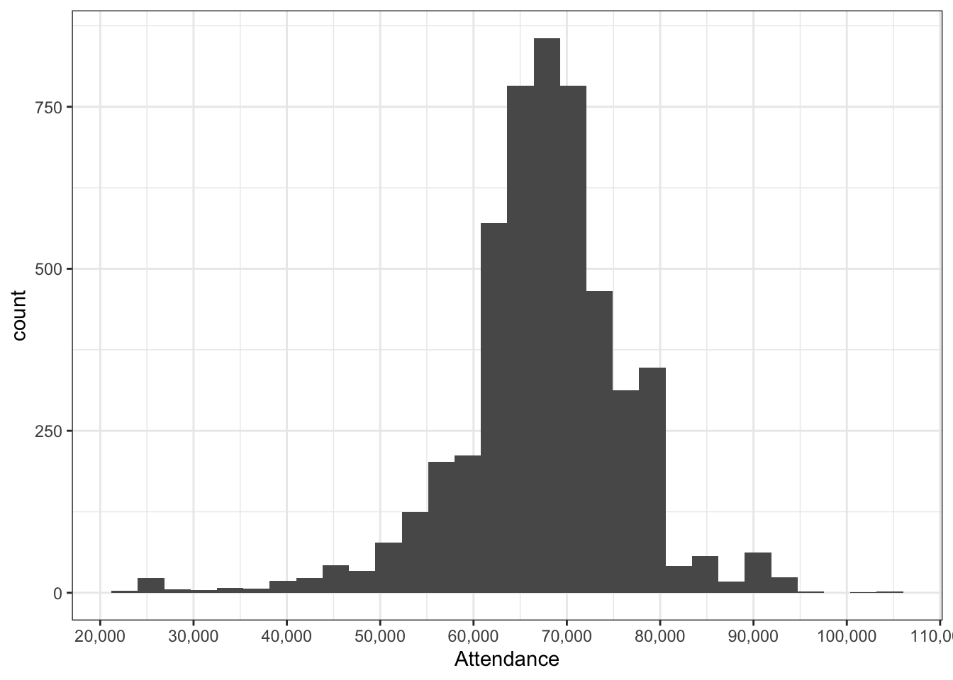
Attendance looks fairly normally distributed, averaging around 70,000 people

Let’s look at attendance by year and by week

nfl_tidy |>
  ggplot(aes(x = weekly_attendance, y = fct_rev(factor(year)))) +
  geom_boxplot() +
  scale_x_continuous(labels = scales::label_comma(), n.breaks = 10) +
  labs(
    x = "Attendance",
    y = NULL
  )

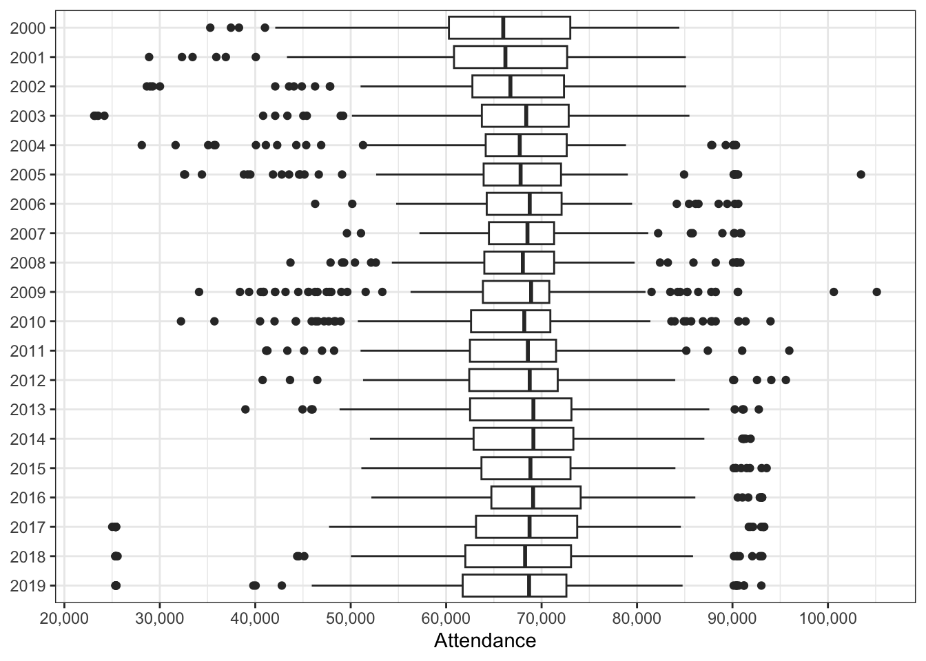
Attendance over the last 20 years is fairly stable, with perhaps a gradual increase over time.

nfl_tidy |>
  ggplot(aes(x = weekly_attendance, y = fct_rev(factor(week)))) +
  geom_boxplot() +
  scale_x_continuous(labels = scales::label_comma(), n.breaks = 10) +
  labs(
    x = "Attendance",
    y = "Week"
  )

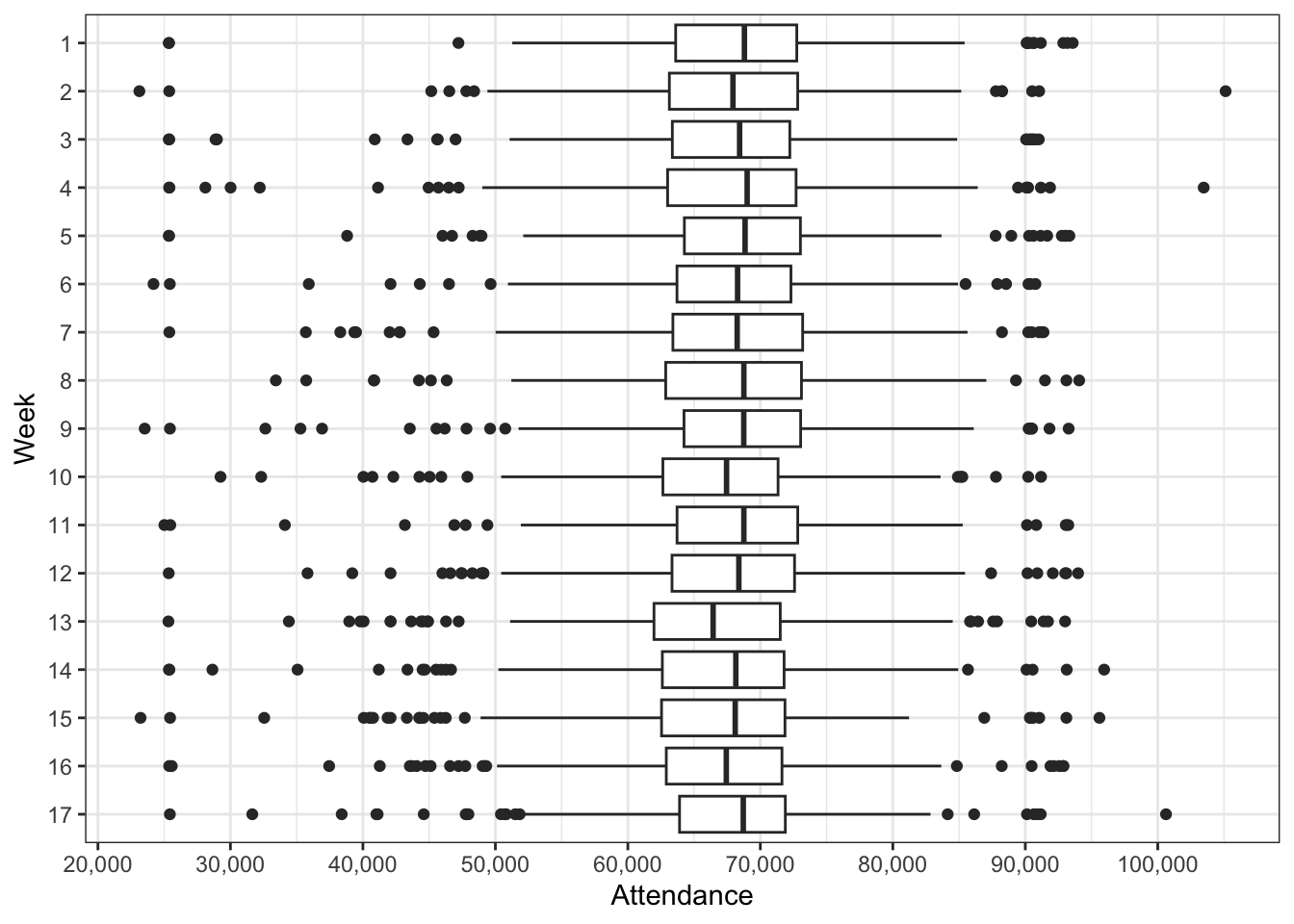
Attendance across the season looks very stable as well.

Home Team

Let’s explore what is probably the biggest factor in game attendance: Home Team

# create function since we will make this plot a few times
attendance_boxplots <- function(data, x, y, fill, n.breaks = 9, labels = scales::label_comma()) {
  data |>
    ggplot(aes({{ x }}, {{ y }}, fill = {{ fill }})) +
    geom_boxplot() +
    scale_x_continuous(labels = labels, n.breaks = n.breaks) +
    expand_limits(x = 0) +
    labs(
      y = NULL,
      x = "Attendance",
      fill = "Conference"
    ) +
    theme(legend.position = "bottom")
}

nfl_tidy |>
  mutate(
    med_attendance = median(weekly_attendance),
    .by = home_team
  ) |>
  mutate(home_team = fct_reorder(word(home_team, -1), med_attendance)) |> # reorder by median attendance
  attendance_boxplots(weekly_attendance, home_team, conference_home_team) +
  ylab("Home Team")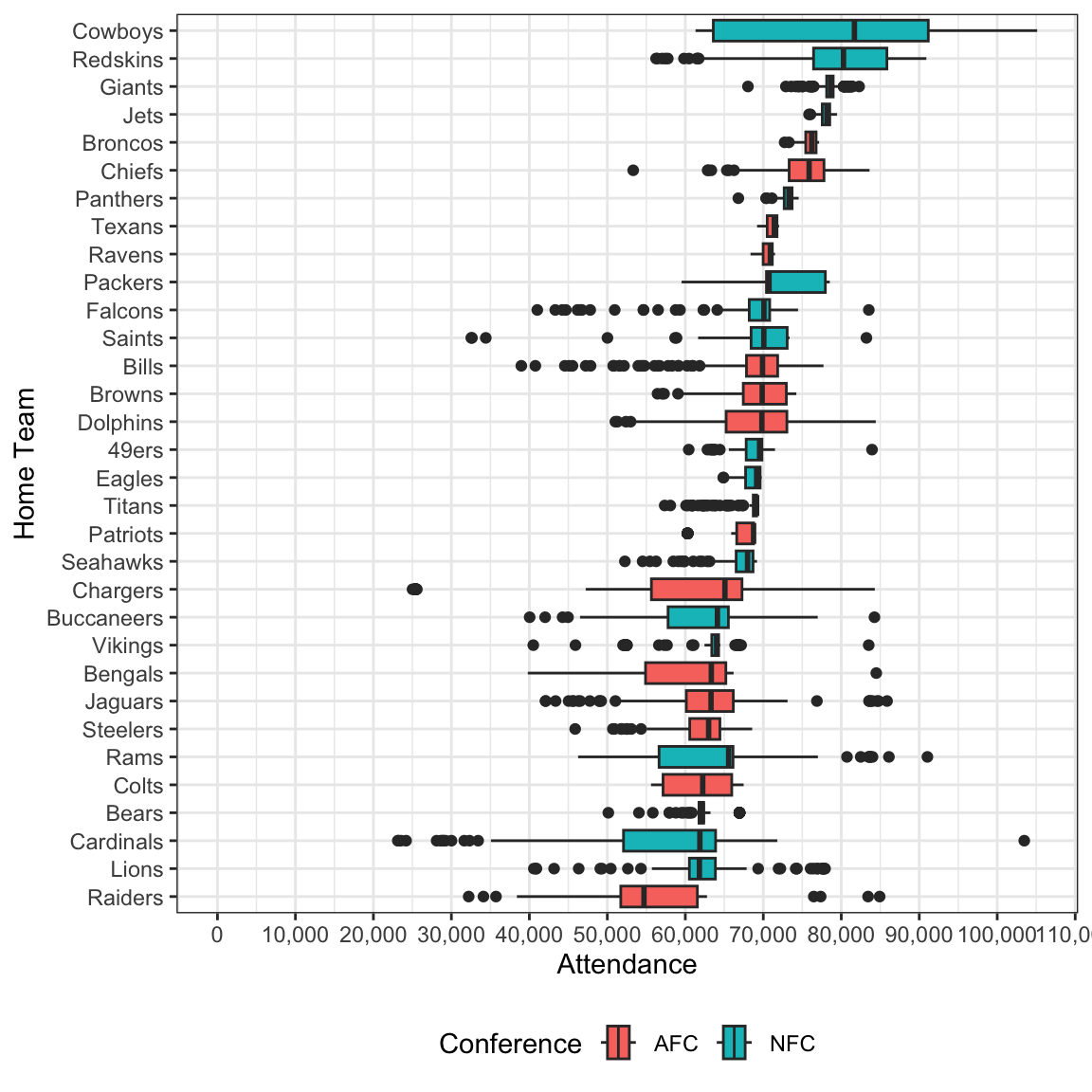

This gives us view into team popularity, but we also need to take into account a glaring confounding variable - stadium capacity.

Stadium Capacity

Let’s now visualize attendance as a percent of stadium capacity.

nfl_tidy |>
  mutate(
    prop_capacity = weekly_attendance / stadium_capacity
  ) |>
  mutate(
    med_prop_capacity = median(prop_capacity, na.rm = T),
    .by = home_team
  ) |>
  mutate(home_team = fct_reorder(word(home_team, -1), med_prop_capacity)) |> # reorder by median attendance
  attendance_boxplots(prop_capacity, home_team, conference_home_team, labels = scales::label_percent()) +
  ylab("Home Team")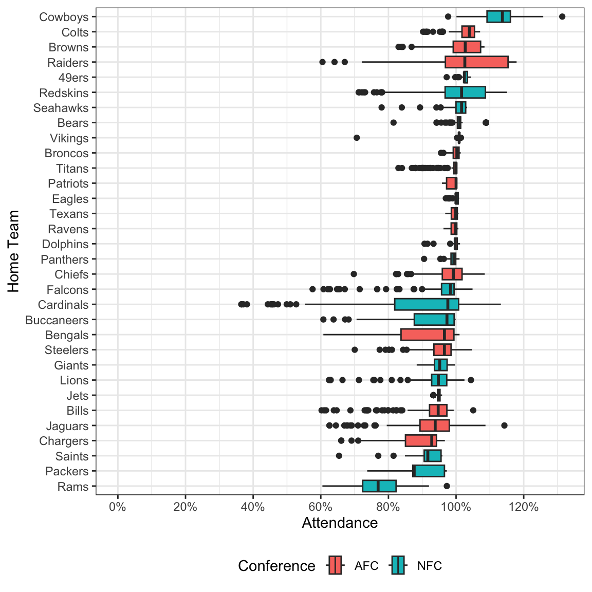

A few things we learn from this chart:

1. Stadiums regularly fill to above capacity

2. While the cowboys still dominate in this regard, unexpected teams such as the Raiders jumped from dead last in terms of nominal attendance to near the top in percent capacity filled. This confirms our suspicion that stadium size plays a part in game attendance.

Away Team

One last related variable we will explore that will reveal some insight is how the away team affects attendance. This stat is not biased by stadium size since away teams play across many stadiums, and may reveal patterns about how widespread a team’s fans are across the country.

nfl_tidy |>
  mutate(
    med_attendance = median(weekly_attendance),
    .by = away_team
  ) |>
  mutate(away_team = fct_reorder(word(away_team, -1), med_attendance)) |> # reorder by median attendance

  attendance_boxplots(weekly_attendance, away_team, conference_away_team) +
  ylab("Away Team")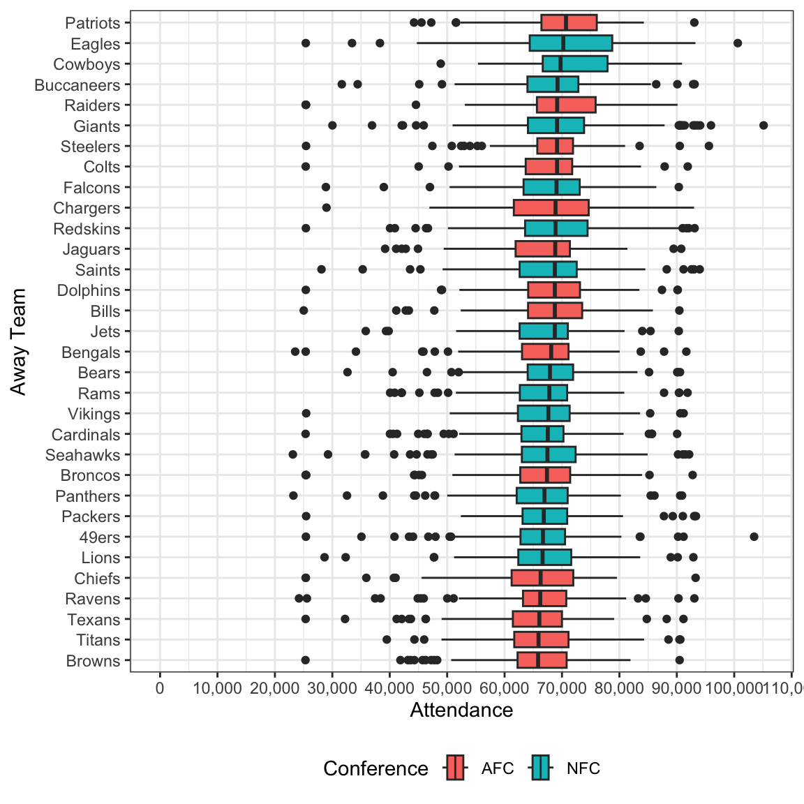

Not unsurprisingly, away teams do not have as much of an affect on attendance as home teams. Nonetheless, It makes sense that the Patriots are a team that many people across the country enjoy seeing their home team play, regardless of whether they love or hate them.

Distance Between Teams

Let’s focus more on a logistical variable: Distance between teams. We might hypothesize that teams further away from each other have smaller attendances.

# Create tibble of team location coordinates
team_locations <-
  nfl_tidy |>
  # add in number of times played at each stadium per season
  add_count(home_team, year, stadium) |>
  # replace stadium with stadium they played at the most that year
  mutate(stadium = stadium[which.max(n)], .by = c(home_team, year)) |>
  distinct(year, team = home_team, stadium) |>
  left_join(
    stadiums |>
      select(stadium, stadium_latitude, stadium_longitude)
  )

# join in team locations twice - once for home team and once for away team
nfl_tidy_with_distances <-
  nfl_tidy |>
  left_join(
    team_locations |>
      select(home_team = team, year, home_team_latitude = stadium_latitude, home_team_longitude = stadium_longitude)
  ) |>
  left_join(
    team_locations |>
      select(away_team = team, year, away_team_latitude = stadium_latitude, away_team_longitude = stadium_longitude)
  ) |>
  rowwise() |>
  # use haversine formula to calculate distance and convert to miles
  mutate(distance_between_teams = geosphere::distHaversine(c(home_team_longitude, home_team_latitude), c(away_team_longitude, away_team_latitude)) / 1609)

nfl_tidy_with_distances |>
  mutate(same_conference = conference_home_team == conference_away_team) |>
  ggplot(aes(distance_between_teams, weekly_attendance)) +
  geom_point(aes(color = same_conference), alpha = .8) +
  geom_smooth() +
  expand_limits(x = 0, y = 0) +
  scale_y_continuous(labels = scales::label_comma(), n.breaks = 10) +
  scale_x_continuous(labels = scales::label_comma(), n.breaks = 10) +
  labs(
    x = "Distance between Teams (mi)",
    y = "Attendance",
    color = "Same Conference"
  )

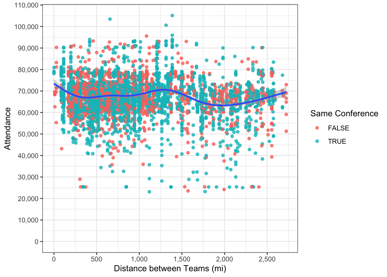
At a glance, there doesn’t appear to be a strong association between distance between teams and attendance, but we won’t write it off since there are so many confounding variables that are baked into the data.

Temperature

How sensitive are fans are about outside temperature? This could be interesting considering there are some stadiums that have retractable ceilings

nfl_tidy |> 
  drop_na(stadium_type) |> 
  ggplot(aes(weather_temperature, weekly_attendance)) + 
  geom_point(aes(color = stadium_type), alpha = .7, show.legend = F) +
  geom_smooth() +
  expand_limits(x = 0, y = 0) +
  scale_y_continuous(labels = scales::label_comma(), n.breaks = 10) +
  facet_wrap(~stadium_type, labeller = "label_both") +
  labs(
    x = "Temperature (F)",
    y = "Attendance"
  )

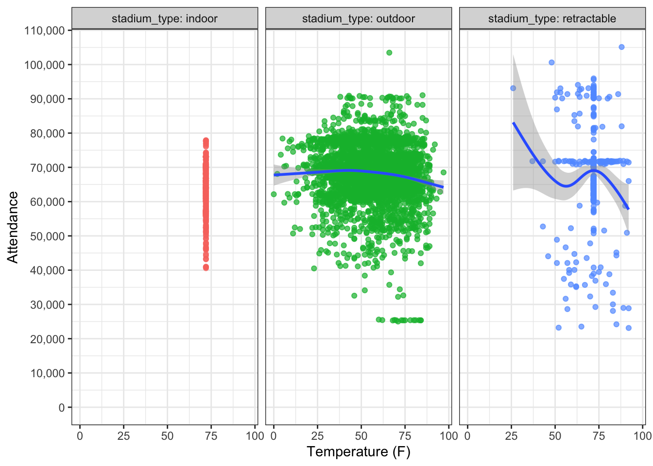
A few things we learn from this chart:

1. I mistakenly believed the temperature data always recorded outside the stadiums
2. There is weak evidence that hotter temperatures lead to lower attendance.

Winning/Losing Streaks

The last association we’ll look at is how past team performance affects attendance. It seems likely that if a home team is on a long winning streak, their fans might be more enthusiastic about attending games. The reverse might also be true about losing streaks, so we will visualize that too.

In order to accomplish this, we will combine winning and losing streaks into a single variable where positive values indicate a winning streak and negative values indicate a losing streak.

nfl_tidy |>
  mutate(
    streak_home_team = if_else(win_streak_home_team == 0, lose_streak_home_team * -1, win_streak_home_team),
    streak_away_team = if_else(win_streak_away_team == 0, lose_streak_away_team * -1, win_streak_away_team)
  ) |>
  pivot_longer(
    c(streak_home_team, streak_away_team),
    names_to = "streak_type",
    values_to = "streak"
  ) |>
  mutate(streak_type = snakecase::to_title_case(streak_type)) |>
  ggplot(aes(streak, weekly_attendance, color = streak_type)) +
  geom_point() +
  geom_smooth() +
  expand_limits(y = 0) +
  scale_y_continuous(labels = scales::label_comma(), n.breaks = 10) +
  labs(
    color = NULL,
    y = "Attendance",
    x = "Streak"
  )

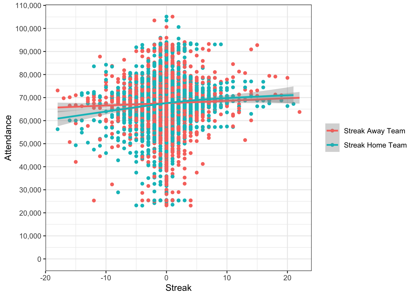
Again, we only see mild effect on attendance, with perhaps a slightly higher affect for home team streaks. However, as with before we won’t write this off completely since there are so many within-group interactions happening which are difficult to visualize.

Up Next

I’ve selected just a few different ways to visualize these data but there are undoubtedly countless more ways. I would love to hear more ideas from you about how to visualize the data!